Section 3 Causality, Subsets, Conditional Statements and Factors
3.1 Experimental Research Design: Racial Discrimination in the Labor Market
Does racial discrimination exist in the labor market? Or should racial disparities in the unemployment rate be attributed to other factors, such as racial gaps in educational attainment? To answer this question, two social scientists (Bertrand and Mullainathan, 2004) conducted the following experiment. In response to newspaper ads, the researchers sent out resumes of fictitious job candidates to potential employers. They varied only the names of the job applicants while leaving the other information in the resumes unchanged. For some resumes, stereotypically African American–sounding names such as Lakisha Washington or Jamal Jones were used, whereas other resumes contained typically White-sounding names such as Emily Walsh or Greg Baker. The researchers then compared the callback rates between these two groups of resumes and examined whether the resumes with stereotypically African American names received fewer callbacks than those with stereotypically White names. The positions to which the applications were sent were either in sales, administrative support, clerical, or customer services.
Let’s examine the data from this experiment in detail. First, we will load some required packages.
# load required packages
library("tidyverse")
library("stringr") # The stringr package provides a cohesive set of functions designed to make working with strings (text or alphanumeric data) easier.
Load in the data resume from the qss package.
Let’s start with some data exploration.
# Retrieve the dimensions of an object (e.g., the number of rows [observations] and columns [variables]).
dim(resume)
## [1] 4870 4## firstname sex race call
## 1 Allison female white 0
## 2 Kristen female white 0
## 3 Lakisha female black 0
## 4 Latonya female black 0
## 5 Carrie female white 0
## 6 Jay male white 0## firstname sex race call
## 4865 Lakisha female black 0
## 4866 Tamika female black 0
## 4867 Ebony female black 0
## 4868 Jay male white 0
## 4869 Latonya female black 0
## 4870 Laurie female white 0## Rows: 4,870
## Columns: 4
## $ firstname <chr> "Allison", "Kristen", "Lakisha", "Latonya", "Carrie", "Jay",…
## $ sex <chr> "female", "female", "female", "female", "female", "male", "f…
## $ race <chr> "white", "white", "black", "black", "white", "white", "white…
## $ call <int> 0, 0, 0, 0, 0, 0, 0, 0, 0, 0, 0, 0, 0, 0, 0, 0, 0, 0, 0, 0, …## firstname sex race call
## Length:4870 Length:4870 Length:4870 Min. :0.00000
## Class :character Class :character Class :character 1st Qu.:0.00000
## Mode :character Mode :character Mode :character Median :0.00000
## Mean :0.08049
## 3rd Qu.:0.00000
## Max. :1.00000We can now start addressing the question of whether resumes with African American–sounding names are less likely to receive callbacks. First, let’s calculate the overall callback rate for the entire dataset using the summarise() function. The purpose of summarise() is to calculate summary statistics (e.g., mean and median) based on the data. This calculation will be important later for assessing whether the average callback rate by race is lower or higher than the overall mean for all candidates.
##    call_back
## 1 0.08049281
Alternatively, you can directly employ the mean() function with the dollar sign ($) using Base R. The dollar sign ($) operator is used to access specific variables or elements within data frames or lists.
## [1] 0.08049281From the total pool of candidate applications, we observe that 8% of the candidates received a callback.
Now, we want to know how many resumes with African American–sounding names received a callback and how many did not. We also want to know the same about the resumes with White-sounding names. In the tidyverse, we can do this with the group_by() function to subset the data by race and callback status. When data is grouped using group_by(), subsequent operations such as summarise(), mutate(), and others, act on individual groups rather than the entire dataset. Hence, after utilizing group_by() it is recommended to conclude the chain of operations with to revert the effects of grouping.
In the code below, after group_by(), we use the count() function to count the number of observations in each subset. The count() function creates a new variable in the data, n, which is the number of observations in that group.
race.call.summary <- resume %>%  # create group for each race and callback status
  group_by(race, call) %>%   # group the data by 'race' and 'call'
  count() %>%  # creates the new variable n, i.e., the number of observations in each group
  ungroup() # remove or revert grouping specifications

race.call.summary
## # A tibble: 4 × 3
## race call n
## <chr> <int> <int>
## 1 black 0 2278
## 2 black 1 157
## 3 white 0 2200
## 4 white 1 235Alternatively, you can use the Base R table() function to create a table that compares the count of black applicants to white applicants who did and did not receive a call back. Additionally, we will label the rows of the table as “race” and the columns as “call”. This kind of table is referred to as a frequency table (also known as a contingency table or a cross-tabulation). It summarizes the count of occurrences of different categorical variables or combinations of variables in a tabular format. The resulting table provides a quick overview of the distribution among the categorical variables.
##        call
## race       0    1
##   black 2278  157
##   white 2200  235
If we want to calculate callback rates (which are callback proportions represented as percentages) based on race, we can use the mutate() function within tidyverse. This function is used to create or modify columns (variables) within a data frame.
(Note: In the tidyverse framework, both mutate() and summarise() are functions used for data manipulation, but they serve distinct purposes. mutate() is employed to create or modify variables within a data set, while maintaining the same number of rows as the original data. This is useful for tasks like data cleaning and variables creation. On the other hand, summarise() is usually used in conjunction with group_by() to aggregate data within defined groups, producing summary values for each group. The basic idea behind summarise() is to collapse multiple rows of data into a single row or a few rows, where the new rows represent a summary of the data such as means, medians, or counts.)
race_call_rate <- race.call.summary %>% # take the data frame race_call_tab and starts a chain of operations using the %>% (pipe) operator.
  group_by(race) %>% # group the data by the 'race' column, preparing for aggregated calculations within each group.
  mutate(call_rate =  n / sum(n)) %>% # calculate the call rate by dividing the number of occurrences ('n') by the sum of 'n' in that group.
  filter(call == 1) %>% # filter the data to keep only the rows where the 'call' column is equal to 1.
  select(race, call_rate) %>%  # select only the 'race' and 'call_rate' columns from the filtered data.
  ungroup() # remove or revert grouping specifications

# Print your data
race_call_rate
## # A tibble: 2 × 2
## race call_rate
## <chr> <dbl>
## 1 black 0.0645
## 2 white 0.0965The callback rate for African Americans was 0.064 or 6% (below the mean) while for Whites it was 0.097 or 10% (above the mean).
We can now compute the causal effect, which refers to the difference in callback rates between resumes with African American–sounding names and those with White-sounding names. It’s important to note that the code below employs = and == for distinct purposes. In R, = can be used for assignment (though <- is recommended), while == is used for evaluating equality between values, comparing the values on its left and right sides for equivalence. (More on conditional statements in Section 3.2.)
race_call_causal <- race_call_rate %>%
  summarize(causal_effect = call_rate[race == "white"] -
  call_rate[race == "black"]) %>%
  pull(causal_effect) # turning tibble into a single number (extracting the numeric value of causal_effect)

race_call_causal
## [1] 0.03203285The racial callback gap (our causal effect) is about 0.032, or 3.2 percentage points. Therefore, our analysis shows that the resumes with an African American–sounding name is less likely to receive a callback than an identical resume with a White-sounding name. While we do not know whether this is the result of intentional discrimination, the lower callback rate for African American job applicants suggests the existence of racial discrimination in the labor market.
3.2 Subsetting Data in R
Now, let’s explore efficient ways to subset data in R.
First, we will create a subset of all individuals whose race variable equals black in the resume data set using the filter() function, i.e., we will extract certain rows from our data frame based on our condition (in this case, when race==“black” is TRUE).
## Rows: 2,435
## Columns: 4
## $ firstname <chr> "Lakisha", "Latonya", "Kenya", "Latonya", "Tyrone", "Aisha",…
## $ sex       <chr> "female", "female", "female", "female", "male", "female", "f…
## $ race      <chr> "black", "black", "black", "black", "black", "black", "black…
## $ call      <int> 0, 0, 0, 0, 0, 0, 0, 0, 0, 0, 0, 0, 0, 0, 0, 0, 0, 0, 0, 0, …
To verify whether everything went well, we can calculate the callback rate for individuals when the value of race is “black.” As calculated in the previous section, this value should be 0.0645.
##    call_rate
## 1 0.06447639
We got it right!
You can also combine the filter() and select() functions with multiple conditions. For example, to keep the call and firstname variables for female individuals with stereotypical black names, we can run the following code,
resumeBf <- resume %>%
  filter(race == "black", sex == "female") %>% # filter rows with race=="black" and sex=="female"
  select(call, firstname)  # keeping only columns call and firstname

head(resumeBf)
## call firstname
## 1 0 Lakisha
## 2 0 Latonya
## 3 0 Kenya
## 4 0 Latonya
## 5 0 Aisha
## 6 0 AishaWe can also calculate the gender gap by group. For this, we first group_by() the data by race and sex and, then, calculate the callback rate for each of the groups:
## `summarise()` has grouped output by 'race'. You can override using the
## `.groups` argument.## # A tibble: 4 × 3
## race sex call
## <chr> <chr> <dbl>
## 1 black female 0.0663
## 2 black male 0.0583
## 3 white female 0.0989
## 4 white male 0.0887The message “summarise() has grouped output by ‘race’. You can override using the .groups argument.” is just a friendly warning message about the resulting grouping structure, and there is nothing wrong with your code.
For a clearer visualization of the information extracted, you can use the spread() function to generate separate columns for each race value. The spread() function is employed to convert data from a “long” format to a “wide” format. (During our Week 3 class, we examined an alternative method to achieve the same outcome using the pivot_wider() function. If you require a review of this approach, consult the Week 3 slides. I find the code using the spread() function to be simpler compared to using pivot_wider().)
resume_sex <- resume_race_sex %>%
  spread(race, call) # creating separate columns for each unique value in the race column, and fills the cells of these columns with the corresponding call values.

resume_sex
## # A tibble: 2 × 3
## sex black white
## <chr> <dbl> <dbl>
## 1 female 0.0663 0.0989
## 2 male 0.0583 0.0887Now we can calculate the differences in callback rates (creating a new variable call_diff) by race and sex.
## # A tibble: 2 × 4
##   sex     black  white call_diff
##   <chr>   <dbl>  <dbl>     <dbl>
## 1 female 0.0663 0.0989    0.0326
## 2 male   0.0583 0.0887    0.0304
All this could be combined into a single chain of operations using only six lines of code. :)
resume %>%
  group_by(race, sex) %>%
  summarise(call = mean(call)) %>%
  ungroup() %>%
  spread(race, call) %>%
  mutate(call_diff = white - black)
## `summarise()` has grouped output by 'race'. You can override using the
## `.groups` argument.## # A tibble: 2 × 4
## sex black white call_diff
## <chr> <dbl> <dbl> <dbl>
## 1 female 0.0663 0.0989 0.0326
## 2 male 0.0583 0.0887 0.0304Alternatively, we could have combined summarise() with the diff() function. The diff() function is used to calculate the differences between consecutive elements in a numeric vector or column of a data frame. In the code below, we use the arrange() function to reorder the rows of the data frame (or tibble) based on the values in one or more columns. This reordering allows you to analyse or visualize data in a more structured and meaningful way.
resume %>%
group_by(race, sex) %>% # group the "resume" data set by "race" and "sex"
summarise(call = mean(call)) %>% # calculate the mean "call" value for each group
group_by(sex) %>% # group the results from the previous step by "sex"
arrange(race) %>% # reorder the rows based on the values of "race"
summarise(call_diff = diff(call)) %>% # compute the differences in the "call" mean values within each "sex" group
ungroup() # remove any grouping applied to the data## `summarise()` has grouped output by 'race'. You can override using the
## `.groups` argument.## # A tibble: 2 × 2
## sex call_diff
## <chr> <dbl>
## 1 female 0.0326
## 2 male 0.03043.3 Conditional Statements
R has a special representation of the two logical values, TRUE and FALSE, which belong to the object class logical.
## [1] "logical"These logical values can be converted into a binary variable in the integer class using the function as.integer(), where TRUE is recoded as 1 and FALSE becomes 0.
## [1] 1## [1] 0In many cases, R will coerce logical values into a binary variable so that performing numerical operations is straightforward. For example, in order to compute the proportion of _TRUE_s in a vector, one can simply compute the sample mean of a logical vector using the mean() function. Similarly, we can sum this vector to compute the total number of _TRUE_s using the sum() function.
## [1] 0.6666667## [1] 2Logical values are often produced with the logical operators & and |, corresponding to logical conjunction (“AND”) and logical disjunction (“OR”), respectively. The value of AND (&) is TRUE only when both of the objects have a value of TRUE.
## [1] FALSE## [1] TRUEThe OR (|) operator is used in a similar way. However, unlike AND, OR is true when at least one of the objects has the value TRUE.
## [1] TRUE## [1] FALSETable 3.1 below summarises these relationships. For example, if one statement is FALSE and the other is TRUE, then the logical conjunction of the two statements is FALSE but their logical disjunction is TRUE (the second and third rows of the table).
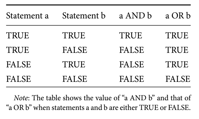
Figure 3.1: Logical Conjunction “AND” and Disjunction “OR”
The package dlpyr within tidyverse has three conditional statement functions if_else(), recode() and case_when.
The if_else() function is allows you to perform conditional operations in a vectorized manner. It’s particularly useful when you need to replace values in a column based on a condition. The function works by evaluating a logical condition for each element of a vector, and if the condition is TRUE, it returns a specified value; otherwise, it returns another value.
The recode() function is a handy way to replace specific values in a vector with new values. Instead of writing multiple if_else() statements for individual replacements, you can achieve the same effect more succinctly with recode(). It takes a vector and replaces specified values with the desired replacements.
The case_when() function is a tool for handling multiple conditions and outcomes. It allows you to define a series of conditions along with the corresponding values to be returned. This function is particularly useful when you have complex conditions that require different outcomes based on different scenarios.
First, let’s create a variable BlackFemale using if_else() and confirm it is only equal to 1 for black and female observations. Two common operators used for building logical conditions in R are the AND operator (&) and the OR operator (|). The AND operator (&) is used to combine two or more conditions, and the result is TRUE only if all the combined conditions are TRUE. The OR operator (|) is used to combine two or more conditions, and the result is TRUE if at least one of the combined conditions is TRUE.
In the code below, we are creating a new data set resume_BlackFemale, by adding a new column called “BlackFemale” to our data set, resume, based on the following conditions: if both conditions “race” is black AND “sex” is female are TRUE, then R will assign a value of 1 to this new column. Otherwise, if FALSE (i.e., if either or both of these conditions are not met), then R will assign a value of 0 to the new column.
resume_BlackFemale <- resume %>%
mutate(BlackFemale = if_else(race == "black" &
sex == "female", 1, 0)) %>%
group_by(BlackFemale, race, sex) %>% # grouping the data based on specified columns
count() # and then performing a count of occurrences within those groups
resume_BlackFemale## # A tibble: 4 × 4
## # Groups: BlackFemale, race, sex [4]
## BlackFemale race sex n
## <dbl> <chr> <chr> <int>
## 1 0 black male 549
## 2 0 white female 1860
## 3 0 white male 575
## 4 1 black female 18863.4 Factor Variables
As we learned in the previous section, the function case_when() is a generalization of the if_else() function to multiple conditions. For example, the code below creates categories for all combinations of race and sex.
resume_categories <- resume %>%
mutate(
race_sex = case_when(
race == "black" & sex == "female" ~ "black female",
race == "white" & sex == "female" ~ "white female",
race == "black" & sex == "male" ~ "black male",
race == "white" & sex == "male" ~ "white male"
)
)
head(resume_categories)## firstname sex race call race_sex
## 1 Allison female white 0 white female
## 2 Kristen female white 0 white female
## 3 Lakisha female black 0 black female
## 4 Latonya female black 0 black female
## 5 Carrie female white 0 white female
## 6 Jay male white 0 white maleIn the above code, within the mutate() function, the case_when() function is employed to establish different conditions that determine the values to be assigned to the race_sex column. Each condition consists of a formula-like structure with a left-hand side and a right-hand side, separated by the “tilde” symbol (~). The left-hand side of each condition defines a logical expression involving the race and sex columns. When a condition is met, it triggers the assignment of a corresponding value to the race_sex column. For example, if the condition race == "black" & sex == "female" is met, the value black female will be assigned to the race_sex column.
Note: The order of the conditions matters. R processes the conditions in sequence, and the first condition that evaluates as true determines the assigned value. Therefore, if multiple conditions could potentially be satisfied for an observation, the value corresponding to the first matching condition will be assigned.
Alternatively, we can create the race_sex variable by using string manipulation functions. For example, we can utilize the mutate() function in conjunction with str_to_title() to capitalize sex and race, and complement this with the str_c function to concatenate these vectors.
resume_race_sex <- resume %>%
mutate(race_sex = str_c(str_to_title(race),
str_to_title(sex)))
head(resume_race_sex)## firstname sex race call race_sex
## 1 Allison female white 0 WhiteFemale
## 2 Kristen female white 0 WhiteFemale
## 3 Lakisha female black 0 BlackFemale
## 4 Latonya female black 0 BlackFemale
## 5 Carrie female white 0 WhiteFemale
## 6 Jay male white 0 WhiteMaleWe can also create a new variable named avg_call to denote the average callback rate for each category within the race_sex variable. This can be achieved through the use of functions group_by(), summarize(), and mean().
## `summarise()` has grouped output by 'race'. You can override using the
## `.groups` argument.
## # A tibble: 4 × 3
## # Groups: race [2]
## race sex avg_call
## <chr> <chr> <dbl>
## 1 black female 0.0663
## 2 black male 0.0583
## 3 white female 0.0989
## 4 white male 0.0887The advantage of this approach is that it eliminates the need for initially creating the factor variable, as demonstrated in the QSS book. For instance, this approach
We can also calculate the callback proportion per firstname, with the option to employ the arrange() function to sort the values in ascending order.
## # A tibble: 36 × 2
##    firstname   call
##    <chr>      <dbl>
##  1 Aisha     0.0222
##  2 Rasheed   0.0299
##  3 Keisha    0.0383
##  4 Tremayne  0.0435
##  5 Kareem    0.0469
##  6 Darnell   0.0476
##  7 Tyrone    0.0533
##  8 Hakim     0.0545
##  9 Tamika    0.0547
## 10 Lakisha   0.055
## # ℹ 26 more rows