Section 5 Observational Studies: Causal Effects and the Counterfactual
5.1 Minimun Wage and Unemployment
Two social science researchers (Card and Krueger, 1994) examined the impact of raising the minimum wage on employment in the fast-food industry. In 1992, the state of New Jersey (NJ) in the United States raised the minimum wage from $4.25 to $5.05 per hour. Did the increase in minimum wage reduce employment, as some economic theories predict? As we discussed in class, answering this question requires inference about the NJ employment rate in the absence of such a raise in minimum wage. Since this counterfactual outcome is not observable, we must somehow estimate it using observed data.
One possible strategy is to look at another state in which the minimum wage did not increase. For example, the researchers of this study chose the neighboring state, Pennsylvania (PA), on the grounds that NJ’s economy resembles that of Pennsylvania, and hence the fast-food restaurants in the two states are comparable. Under this cross-section comparison design, therefore, the fast-food restaurants in NJ serve as the treatment group receiving the treatment (i.e., the increase in minimum wage), whereas those in PA represent the control group, which did not receive such a treatment.
To collect pretreatment and outcome measures, the researchers surveyed the fast-food restaurants before and after the minimum wage increase. Specifically, they gathered information about the number of full-time employees, the number of part-time employees, and their hourly wages for each restaurant.
Let’s start loading some necessary packages, the data and inspect the minimum wage data from the qss package:
## Rows: 358
## Columns: 8
## $ chain      <chr> "wendys", "wendys", "burgerking", "burgerking", "kfc", "kfc…
## $ location   <chr> "PA", "PA", "PA", "PA", "PA", "PA", "PA", "PA", "PA", "PA",…
## $ wageBefore <dbl> 5.00, 5.50, 5.00, 5.00, 5.25, 5.00, 5.00, 5.00, 5.00, 5.50,…
## $ wageAfter  <dbl> 5.25, 4.75, 4.75, 5.00, 5.00, 5.00, 4.75, 5.00, 4.50, 4.75,…
## $ fullBefore <dbl> 20.0, 6.0, 50.0, 10.0, 2.0, 2.0, 2.5, 40.0, 8.0, 10.5, 6.0,…
## $ fullAfter  <dbl> 0.0, 28.0, 15.0, 26.0, 3.0, 2.0, 1.0, 9.0, 7.0, 18.0, 5.0, …
## $ partBefore <dbl> 20.0, 26.0, 35.0, 17.0, 8.0, 10.0, 20.0, 30.0, 27.0, 30.0, …
## $ partAfter <dbl> 36, 3, 18, 9, 12, 9, 25, 32, 39, 10, 20, 4, 13, 20, 15, 19,…## chain location wageBefore wageAfter
## Length:358 Length:358 Min. :4.250 Min. :4.250
## Class :character Class :character 1st Qu.:4.250 1st Qu.:5.050
## Mode :character Mode :character Median :4.500 Median :5.050
## Mean :4.618 Mean :4.994
## 3rd Qu.:4.987 3rd Qu.:5.050
## Max. :5.750 Max. :6.250
## fullBefore fullAfter partBefore partAfter
## Min. : 0.000 Min. : 0.000 Min. : 0.00 Min. : 0.00
## 1st Qu.: 2.125 1st Qu.: 2.000 1st Qu.:11.00 1st Qu.:11.00
## Median : 6.000 Median : 6.000 Median :16.25 Median :17.00
## Mean : 8.475 Mean : 8.362 Mean :18.75 Mean :18.69
## 3rd Qu.:12.000 3rd Qu.:12.000 3rd Qu.:25.00 3rd Qu.:25.00
## Max. :60.000 Max. :40.000 Max. :60.00 Max. :60.00First, calculate the proportion of restaurants by state whose hourly wages were less than the minimum wage in NJ, $5.05, for wageBefore and wageAfter:
Since the NJ minimum wage was $5.05, we’ll define a variable with that value. Even if you use them only once or twice, it is a good idea to put values like this in vectors (in this case, a scalar). It makes your code closer to self-documenting, i.e. easier for others (including you, in the future) to understand what the code does.
Later, it will be easier to understand wageAfter < NJ_MINWAGE without any comments than it would be to understand wageAfter < 5.05.
In the latter case you’d have to remember that the new NJ minimum wage was 5.05 and that’s why you were using that value.
Using 5.05 in your code, instead of assigning it to an object called NJ_MINWAGE, is an example of a magic number; try to avoid them.
Note that the variable location has multiple values: PA and four regions of NJ.
So we’ll add a state variable to the data.
##    location   n
## 1        PA  67
## 2 centralNJ  45
## 3   northNJ 146
## 4   shoreNJ  33
## 5   southNJ  67
We can extract the abbreviation for each state by using thestringr() function str_sub(). The value -2L indicates that the substring extraction will start from the second-to-last character and go until the end of the string. Essentially, it’s extracting the last two characters of the location string.
Alternatively, as we did in class, since "PA" is the only value that an observation in Pennsylvania takes in location, and since all other observations are in New Jersey:
Let’s evaluate whether the restaurants in NJ followed the law:
minwage %>%
  group_by(state) %>%
  summarise(prop_after = mean(wageAfter < NJ_MINWAGE),
            prop_Before = mean(wageBefore < NJ_MINWAGE))
## # A tibble: 2 × 3
## state prop_after prop_Before
## <chr> <dbl> <dbl>
## 1 NJ 0.00344 0.911
## 2 PA 0.955 0.940Create a variable for the proportion of full-time employees in NJ and PA after the increase:
minwage <-
  minwage %>%
  mutate(totalAfter = fullAfter + partAfter,
        fullPropAfter = fullAfter / totalAfter)
Now calculate the average proportion of full-time employees for each state:
full_prop_by_state <-
  minwage %>%
  group_by(state) %>%
  summarise(fullPropAfter = mean(fullPropAfter))
full_prop_by_state
## # A tibble: 2 × 2
## state fullPropAfter
## <chr> <dbl>
## 1 NJ 0.320
## 2 PA 0.272We could compute the difference in means between NJ and PA by
(filter(full_prop_by_state, state == "NJ")[["fullPropAfter"]] -
  filter(full_prop_by_state, state == "PA")[["fullPropAfter"]])
## [1] 0.04811886or
## # A tibble: 1 × 3
##      NJ    PA   diff
##   <dbl> <dbl>  <dbl>
## 1 0.320 0.272 0.0481
The results suggest that the restaurants in NJ followed the minimum wage increase law.
5.1.1 Confounding Bias
We can calculate the proportion of each chain out of all fast-food restaurants in each state:
We can easily compare these using a dot-plot:
ggplot(chains_by_state, aes(x = chain, y = prop, colour = state)) +
  geom_point() +
  coord_flip() +
  theme_few()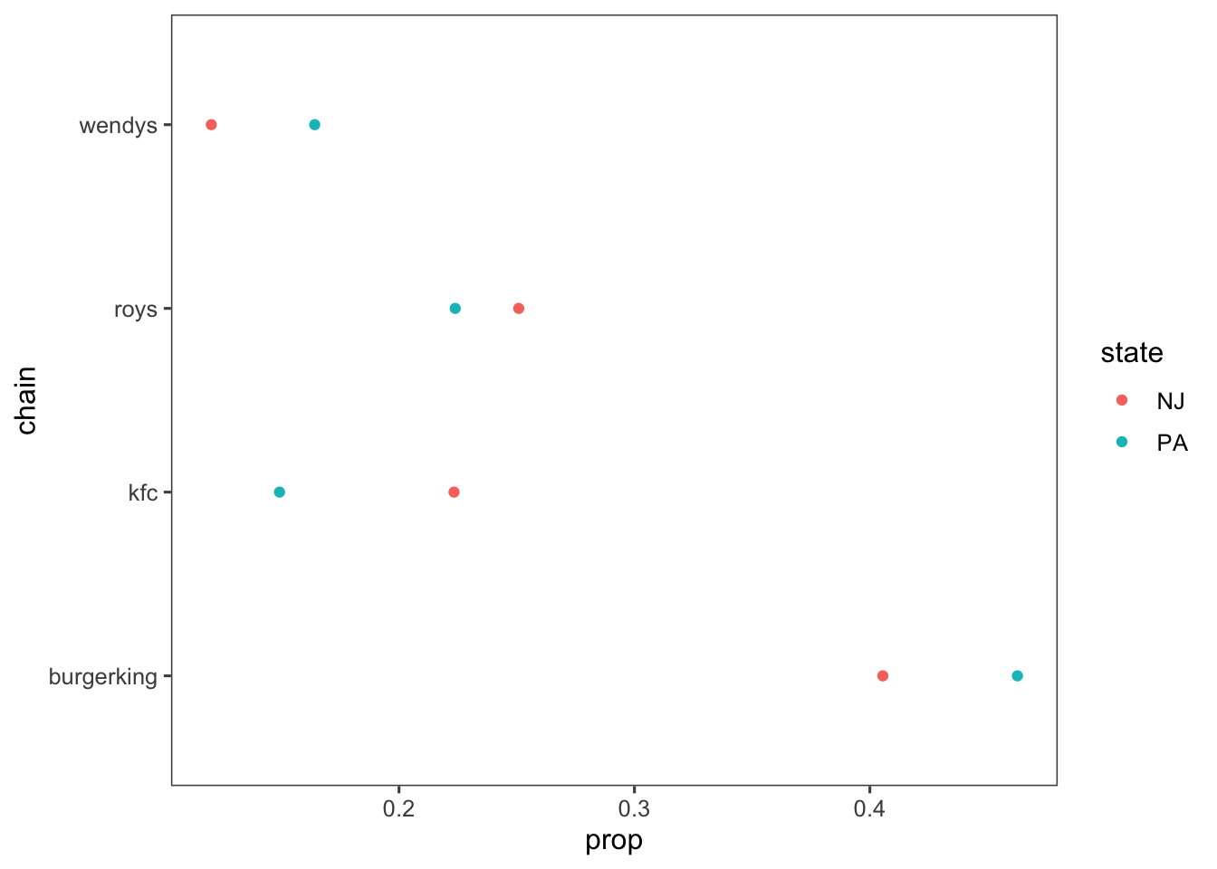
In the QSS text, only Burger King restaurants are compared.
However, tidyverse makes comparing all restaurants not much more complicated than comparing two.
All we have to do is change the group_by statement we used previously so that we group by chain restaurants and state:
full_prop_by_state_chain <-
  minwage %>%
  group_by(state, chain) %>%
  summarise(fullPropAfter = mean(fullPropAfter))
## `summarise()` has grouped output by 'state'. You can override using the
## `.groups` argument.## # A tibble: 8 × 3
## # Groups: state [2]
## state chain fullPropAfter
## <chr> <chr> <dbl>
## 1 NJ burgerking 0.358
## 2 NJ kfc 0.328
## 3 NJ roys 0.283
## 4 NJ wendys 0.260
## 5 PA burgerking 0.321
## 6 PA kfc 0.236
## 7 PA roys 0.213
## 8 PA wendys 0.248We can plot and compare the proportions easily in this format.
In general, ordering categorical variables alphabetically is useless, so we’ll order the chains by the average of the NJ and PA fullPropAfter, using fct_reorder() function (particularly useful for reordering the levels of a factor based on some specific criterion).
ggplot(full_prop_by_state_chain,
       aes(x = fct_reorder(chain, fullPropAfter),
           y = fullPropAfter,
           colour = state)) +
  geom_point() +
  coord_flip() +
  labs(x = "chains") +
  theme_few()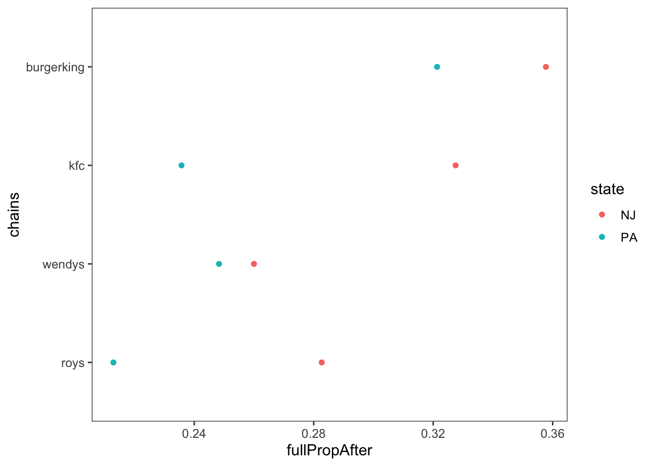
To calculate the difference between states in the proportion of full-time employees after the change:
## # A tibble: 4 × 4
##   chain         NJ    PA   diff
##   <chr>      <dbl> <dbl>  <dbl>
## 1 burgerking 0.358 0.321 0.0364
## 2 kfc        0.328 0.236 0.0918
## 3 roys       0.283 0.213 0.0697
## 4 wendys     0.260 0.248 0.0117
5.1.2 Before and After Analysis
To compute the estimates in the before and after design first create an additional variable for the proportion of full-time employees before the minimum wage increase.
minwage <-
  minwage %>%
  mutate(totalBefore = fullBefore + partBefore,
         fullPropBefore = fullBefore / totalBefore)
The before-and-after analysis is the difference between the full-time employment before and after the minimum wage law passed looking only at NJ:
##         diff
## 1 0.02387474
The result of the before-and-after analysis suggests that the increase in minimum wage had no negative impact on full-time employment. If anything, it appears to have slightly increased the proportion of full-time employment in fast-food restaurants.
The disadvantage of the before-and-after design is that time-varying confounding factors can bias the resulting inference. For example, suppose that there is an upward time trend in the local NJ economy and wages and employment are improving. If this trend is not caused by the minimum wage increase, then we may incorrectly attribute the difference between the two time periods to the raise in minimum wage. The before-and-after design critically rests upon the nonexistence of such time trends.
5.1.3 Difference-in-Difference Research Design
The difference-in-differences design uses the difference in the before-and-after differences for each state. As you remember from class, the counterfactual outcome assumes that New Jersey follows the same trend as Pennsylvania, representing what might have occurred in NJ without the minimum wage increase in NJ.
The average causal effect for NJ’s restaurants is then calculated from the difference between the observed (factual) outcome after the minimum wage increase, and the counterfactual outcome derived under the parallel time trend assumption.
The Difference-in-Differences (DiD) estimate can be expressed as:
\[ \text{DiD estimate} = \underbrace{\left( \overline{Y}_{\text{after treated}} - \overline{Y}_{\text{before treated}} \right)}_{\text{difference for the treatment group}} - \underbrace{\left( \overline{Y}_{\text{after control}} - \overline{Y}_{\text{before control}} \right)}_{\text{difference for the control group}} \] We can now compute the DiD estimate:
minwage %>%
  group_by(state) %>%
  summarise(diff = mean(fullPropAfter) - mean(fullPropBefore)) %>%
  spread(state, diff) %>% # convert data from "long" to "wide"
  mutate(diff_in_diff = NJ - PA)
## # A tibble: 1 × 3
## NJ PA diff_in_diff
## <dbl> <dbl> <dbl>
## 1 0.0239 -0.0377 0.0616The result suggests that the increase in minimum wage had no negative impact on full-time employment. This finding goes against the prediction of some economists that raising the minimum wage has a negative impact on employment. If anything, our DiD analysis suggests that the increase in minimum wage slightly increased (by 6%) the proportion of full-time employment in NJ fast-food restaurants.
Now, let’s create a single dataset with the mean values of each state before and after to visually look at each of these designs. In the code below, the gather() function is used to reshape the data to transform specific columns into two columns: a key column and a value column. In this case: period will be the new column that stores the column names (keys). fullProp will be the new column that stores the corresponding values. -state means that the state column will be left unchanged (it won’t be gathered). So, after this step, for every row in your original data that had separate fullPropAfter and fullPropBefore values, you’ll now have two rows. One row will have period set to fullPropAfter and fullProp set to the corresponding value. The second row will have period set to fullPropBefore and fullProp set to its corresponding value.
full_prop_by_state <-
  minwage %>%
  group_by(state) %>%
  summarise_at(vars(fullPropAfter, fullPropBefore), mean) %>%
  gather(period, fullProp, -state) %>%
  mutate(period = recode(period, fullPropAfter = 1, fullPropBefore = 0))
full_prop_by_state
## # A tibble: 4 × 3
## state period fullProp
## <chr> <dbl> <dbl>
## 1 NJ 1 0.320
## 2 PA 1 0.272
## 3 NJ 0 0.297
## 4 PA 0 0.310Now plot this new dataset:
ggplot(full_prop_by_state, aes(x = period, y = fullProp, colour = state)) +
  geom_point() +
  geom_line() +
  scale_x_continuous(breaks = c(0, 1), labels = c("Before", "After")) +
  theme_few()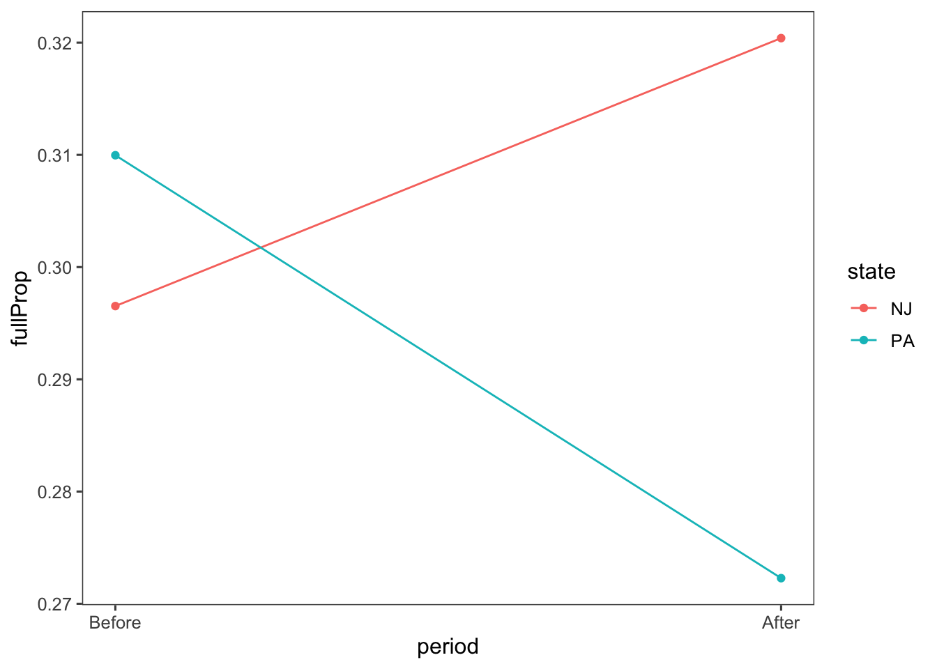
5.2 Descriptive Statistics for a Single Variable
To calculate the summary for the variables wageBefore and wageAfter for New Jersey only:
##    wageBefore     wageAfter
##  Min.   :4.25   Min.   :5.000
##  1st Qu.:4.25   1st Qu.:5.050
##  Median :4.50   Median :5.050
##  Mean   :4.61   Mean   :5.081
##  3rd Qu.:4.87   3rd Qu.:5.050
##  Max.   :5.75   Max.   :5.750
We calculate the interquartile range for each state’s wages after the passage of the law using the same grouped summarize as we used before:
## # A tibble: 2 × 3
##   state wageAfter wageBefore
##   <chr>     <dbl>      <dbl>
## 1 NJ        0           0.62
## 2 PA        0.575       0.75
Calculate the variance and standard deviation of wageAfter and wageBefore for each state:
minwage %>%
  group_by(state) %>%
  summarise(wageAfter_sd = sd(wageAfter),
               wageAfter_var = var(wageAfter),
               wageBefore_sd = sd(wageBefore),
               wageBefore_var = var(wageBefore))
## # A tibble: 2 × 5
## state wageAfter_sd wageAfter_var wageBefore_sd wageBefore_var
## <chr> <dbl> <dbl> <dbl> <dbl>
## 1 NJ 0.106 0.0112 0.343 0.118
## 2 PA 0.359 0.129 0.358 0.128Alternatively, the function summarise() combined with the across() function allows the application of a function (or functions) across multiple columns using multiple functions such as sd() and var() for the calculation of the standard deviation and the variance, respectively.
minwage %>%
  group_by(state) %>%
  summarise(across(c(wageAfter, wageBefore), list(sd = sd, var = var)))
## # A tibble: 2 × 5
## state wageAfter_sd wageAfter_var wageBefore_sd wageBefore_var
## <chr> <dbl> <dbl> <dbl> <dbl>
## 1 NJ 0.106 0.0112 0.343 0.118
## 2 PA 0.359 0.129 0.358 0.128