Book of Codes
POLS8042: Quantitative Research for Political Science
2024-09-24
Section 1 Introduction to R and RStudio
This is the book of codes for the course POLS8042: Quantitative Research for Political Science. This material is heavily based on the required readings for the course.
We will be using RStudio, as it provides an easier way to interact with the R environment. When you open RStudio, you will see the following four windows (also called panes) shown in Figure 1.1 below. However, your windows might be in a different order that those in Figure 1.1. If you’d like, you can change the order of the windows under RStudio preferences. You can also change their shape by either clicking the minimize or maximize buttons on the top right of each panel, or by clicking and dragging the middle of the borders of the windows.
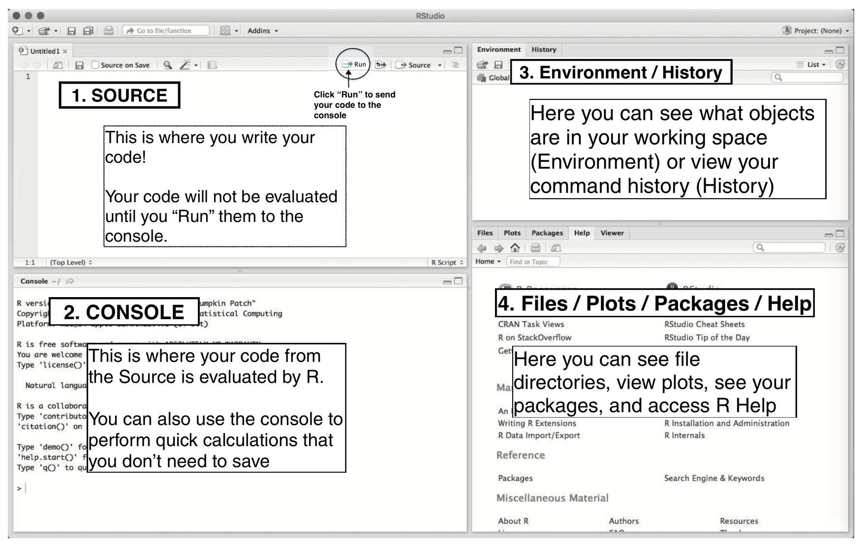
Figure 1.1: The Four RStudio Windows
The four RStudio windows are:
- The upper-left window (Source) displays a script that contains code.
- The lower-left window (Console) shows the console where R commands can be directly entered.
- The upper-right window (Environment/History) lists R objects and a history of executed R commands.
- Finally, the lower-right window (Files/Plots/Packages/Help) enables us to view plots, data sets, files and subdirectories in the working directory, R packages, and help pages.
1.1 Arithmetic Operations
We begin by using R as a calculator with standard arithmetic operators. In figure 1.1, the left-hand window of RStudio shows the R console where we can directly enter R commands. In this R console, we can type in, for example, 5 + 3, then hit Enter on our keyboard (R ignores spaces, and so 5+3 will return the same result).
## [1] 8As this example illustrates, this book displays R commands followed by the outputs they would produce if entered in the R console. These outputs begin with ## to distinguish them from the R commands that produced them, though this mark will not appear in your R console. Also, do not confuse the output with the # (hashtag) character used at the beginning of a line in code. In R, the # symbol is used to denote a comment. Comments are parts of the code that are not executed (i.e., they are not evaluated by the console) and are typically used to provide explanations or context about what the code is doing.
## [1] 8Finally, in this example, [1] indicates that the output is the first element of a vector of length 1. It is important for readers to try these examples on their own. Remember that we can learn programming only by doing! Let’s try other examples.
## [1] 2## [1] 1.666667## [1] 125## [1] 35## [1] 2The final expression sqrt(4) is an example of a so-called function, which takes an input (or multiple inputs) and produces an output. Here, the function sqrt() takes a nonnegative number and returns its square root. R has numerous other functions, and users can even make their own functions.
1.2 Objects
R can store information as an object with a name of our choice. Once we have created an object, we just refer to it by name. That is, we are using objects as “shortcuts” to some piece of information or data. For this reason, it is important to use an intuitive and informative name. The name of our object must follow certain restrictions. For example, it cannot begin with a number (but it can contain numbers). Object names also should not contain spaces. We must avoid special characters such as % and $, which have specific meanings in R. In RStudio, in the upper-right window, called Environment (see figure 1.1), we will see the objects we created. We use the assignment operator <- to assign some value to an object. For example, we can store the result of the above calculation as an object named result, and thereafter we can access the value by referring to the object’s name. By default, R will print the value of the object to the console if we just enter the object name and hit Enter.
## [1] 8Alternatively, we can explicitly print it by using the print() function.
## [1] 8Note that if we assign a different value to the same object name, then the value of the object will be changed. As a result, we must be careful not to overwrite previously assigned information that we plan to use later.
## [1] 2Another thing to be careful about is that object names are case sensitive. For example, Hello is not the same as either hello or HELLO. As a consequence, we receive an error in the R console when we type Result rather than result, which is defined above.
Encountering programming errors or bugs is part of the learning process. The tricky part is figuring out how to fix them. Here, the error message tells us that the Result object does not exist. We can see the list of existing objects in the Environment tab in the upper-right window (see figure 1.1), where we will find that the correct object is result. It is also possible to obtain the same list by using the ls() function.
So far, we have assigned only numbers to an object. But R can represent various other types of values as objects. For example, we can store a string of characters by using quotation marks.
## [1] "instructor"In character strings, spacing is allowed.
## [1] "instructor but not the author of the book"Notice that R treats numbers like characters when we tell it to do so.
## [1] "5"However, arithmetic operations like addition and subtraction cannot be used for character strings. For example, attempting to divide or take a square root of a character string will result in an error.
R recognizes different types of objects by assigning each object to a class. Separating objects into classes allows R to perform appropriate operations depending on the objects’ class. For example, a number is stored as a numeric object whereas a character string is recognized as a character object. In RStudio, the Environment window will show the class of an object as well as its name. The function (which by the way is another class) class() tells us to which class an object belongs.
## [1] 2## [1] "numeric"## [1] "5"## [1] "character"## [1] "function"There are many other classes in R, some of which will be introduced throughout this book. In fact, it is even possible to create our own object classes.
1.3 Vectors
We present the simplest (but most inefficient) way of entering data into R. Table 1.2 contains estimates of world population (in thousands) over the past several decades.
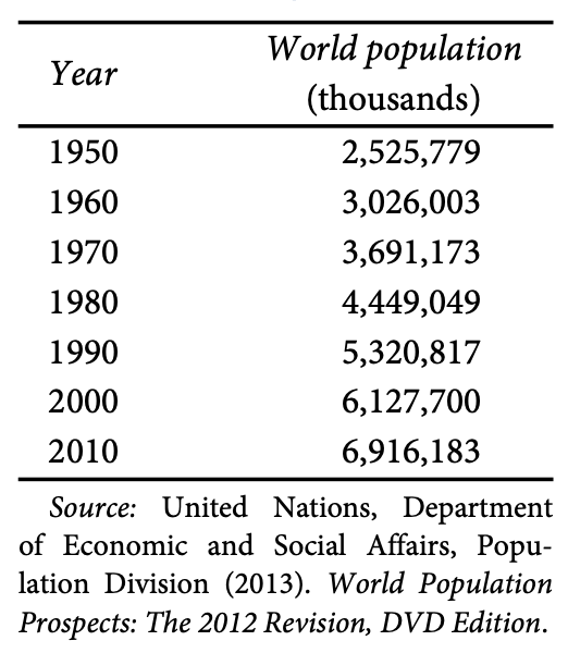
Figure 1.2: World Population Estimates by Decades
We can enter these data into R as a numeric vector object (also called one-dimensional array).
An array is a data structure that can store a collection of items in an organized way. Arrays can have one or more dimensions.
A one-dimensional array is a simple list of elements that can be accessed using a single index.
In the context of R, a vector is a one-dimensional array. It is a basic data structure in R that contains elements of the same type (numeric, character, or logical).
To create a vector in R, we use the c() function, which stands for ‘concatenate.’ This function allows us to combine multiple values into a single vector, with commas separating each element. For example, we can use the c() function to enter world population estimates as elements of a single vector.
## [1] 2525779 3026003 3691173 4449049 5320817 6127700 6916183We also note that the c() function can be used to combine multiple vectors.
pop_first <- c(2525779, 3026003, 3691173)
pop_second <- c(4449049, 5320817, 6127700, 6916183)
pop_all <- c(pop_first, pop_second)
pop_all
## [1] 2525779 3026003 3691173 4449049 5320817 6127700 6916183To access specific elements of a vector, we use square brackets [ ]. This is called indexing. Multiple elements can be extracted via a vector of indices within square brackets. Also within square brackets the dash, -, removes the corresponding element from a vector. Note that none of these operations change the original vector.
## [1] 3026003## [1] 3026003 4449049## [1] 4449049 3026003## [1] 2525779 3026003 4449049 5320817 6127700 6916183Since each element of this vector is a numeric value, we can apply arithmetic operations to it. The operations will be repeated for each element of the vector. Let’s give the population estimates in millions instead of thousands by dividing each element of the vector by 1000.
## [1] 2525.779 3026.003 3691.173 4449.049 5320.817 6127.700 6916.183We can also express each population estimate as a proportion of the 1950 population estimate. Recall that the 1950 estimate is the first element of the vector world_pop.
## [1] 1.000000 1.198047 1.461400 1.761456 2.106604 2.426063 2.738238In addition, arithmetic operations can be done using multiple vectors. For example, we can calculate the percentage increase in population for each decade, defined as the increase over the decade divided by its beginning population. For example, suppose that the population was 100 thousand in one year and increased to 120 thousand in the following year. In this case, we say, “the population increased by 20%.” To compute the percentage increase for each decade, we first create two vectors, one without the first decade and the other without the last decade. We then subtract the second vector from the first vector. Each element of the resulting vector equals the population increase. For example, the first element is the difference between the 1960 population estimate and the 1950 estimate.
## [1] 500224 665170 757876 871768 806883 788483## [1] 19.80474 21.98180 20.53212 19.59448 15.16464 12.86752Finally, we can also replace the values associated with particular indices by using the usual assignment operator (<-). Below, we replace the first two elements of the percent.increase vector with their rounded values.
## [1] 20.00000 22.00000 20.53212 19.59448 15.16464 12.86752Alternatively, we can round the values using the round() function. The first argument of this function is the number you wish to round (in our case, all elements of the percent.increase vector), and the optional second argument specifies the number of decimal places to which you want to round (we will round the values to two decimal places). If you don’t provide the second argument, R will round to the nearest whole number.
## [1] 20.00 22.00 20.53 19.59 15.16 12.871.4 Functions
Functions are important objects in R and perform a wide range of tasks. A function often takes multiple input objects and returns an output object. We have already seen several functions: sqrt(), print(), class(), round(), and c(). In R, a function generally runs as funcname(input) where funcname is the function name and input is the input object. In programming (and in math), we call these inputs arguments. For example, in the syntax sqrt(4), sqrt is the function name and 4 is the argument or the input object.
Some basic functions useful for summarizing data include length() for the length of a vector or equivalently the number of elements it has, min() for the minimum value, max() for the maximum value, range() for the range of data, mean() for the mean, and sum() for the sum of the data. Right now we are inputting only one object into these functions so we will not use argument names.
## [1] 7## [1] 2525779## [1] 6916183## [1] 2525779 6916183## [1] 4579529## [1] 4579529The last expression gives another way of calculating the mean as the sum of all the elements divided by the number of elements.
When multiple arguments are given, the syntax looks like funcname(input1, input2). The order of inputs matters. That is, funcname(input1, input2) is different from funcname(input2, input1). To avoid confusion and problems stemming from the order in which we list arguments, it is also a good idea to specify the name of the argument that each input corresponds to. This looks like funcname(arg1 = input1, arg2 = input2). For example, the seq() function can generate a vector composed of an increasing or decreasing sequence. The first argument from specifies the number to start from; the second argument to specifies the number at which to end the sequence; the last argument by indicates the interval to increase or decrease by. We can create an object for the year variable from table 1.2 using this function.
## [1] 1950 1960 1970 1980 1990 2000 2010Notice how we can switch the order of the arguments without changing the output because we have named the input objects.
## [1] 1950 1960 1970 1980 1990 2000 2010Although not relevant in this particular example, we can also create a decreasing sequence using the seq() function. In addition, the colon operator : creates a simple sequence, beginning with the first number specified and increasing or decreasing by 1 to the last number specified.
## [1] 2010 2000 1990 1980 1970 1960 1950## [1] 2008 2009 2010 2011 2012## [1] 2012 2011 2010 2009 2008The names() function can access and assign names to elements of a vector. Element names are not part of the data themselves, but are helpful attributes of the R object. Below, we see that the object world.pop does not yet have the names attribute, with names(world_pop) returning the NULL value. However, once we assign the year as the labels for the object, each element of world.pop is printed with an informative label.
## NULL## [1] "1950" "1960" "1970" "1980" "1990" "2000" "2010"## 1950 1960 1970 1980 1990 2000 2010
## 2525779 3026003 3691173 4449049 5320817 6127700 6916183In many situations, we want to create our own functions and use them repeatedly. This allows us to avoid duplicating identical (or nearly identical) sets of code chunks, making our code more efficient and easily interpretable. The function() function can create a new function. The syntax takes the following form:
In this example code, myfunction is the function name, input1, input2, …, inputN are the input arguments, and the commands within the braces { } define the actual function. Finally, the return() function returns the output of the function. We begin with a simple example, creating a function to compute a summary of a numeric vector.
my_summary <- function(x){ # function takes one input
  s_out <- sum(x)
  l_out <- length(x)
  m_out <- s_out / l_out
  out <- c(s_out, l_out, m_out) # define the output
  names(out) <- c("sum", "length", "mean") # add labels
  return(out) # end function by calling output
}
Now, let’s generate a simple numeric vector from 1 to 10, called z, to test our new function.
##    sum length   mean
##   55.0   10.0    5.5
Note that objects (e.g., x, s_out, l_out, m_out, and out in the above example) can be defined within a function independently of the environment in which the function is being created. This means that we need not worry about using identical names for objects inside a function and those outside it.
We can also use our numeric vector world_pop as the input for our new function.
##      sum   length     mean
## 32056704        7  4579529
The getAnywhere() function is used to retrieve information about an object, including functions. For instance, we can use getAnywhere() to access the source code of the my.summary() function we just created.
## A single object matching 'my_summary' was found
## It was found in the following places
##   .GlobalEnv
## with value
##
## function(x){ # function takes one input
##   s_out <- sum(x)
##   l_out <- length(x)
##   m_out <- s_out / l_out
##   out <- c(s_out, l_out, m_out) # define the output
##   names(out) <- c("sum", "length", "mean") # add labels
##   return(out) # end function by calling output
## }
## <bytecode: 0x11c0e4a00>
1.5 Programming Style and Learning Tips
Following a consistent coding style is important for your code to be readable by you and others. The preferred style is the tidyverse style guide.
- The lintr package will check files for style errors.
In RStudio, you can go to the Tools > Global Options > Code > Diagnostics pane and check the box Provide R style diagnostics (e.g., whitespace). On the same pane, there are other options that can be set in order to increase or decrease the amount of warnings while writing R code in RStudio.
1.6 Interactive R Learning: Lab 1
swirl is a R package that turns the R console into an interactive learning environment. Swirl stands for “Statistics With Interactive R Learning.” Users receive immediate feedback as they are guided through self-paced lessons in data science and R programming.
Swirl lessons for the book, “Quantitative Social Science: An Introduction” (QSS), are available. Follow the code below to install swirl and start a qss-swirl lesson.
To install the qss-swirl lessons from Github, we first need to install devtools, a package that provides various functions to make installation of packages hosted on GitHub repositories easier.
# Install devtools
install.packages("devtools")

# Install the qss-swirl lessons from github
install_course_github("kosukeimai", "qss-swirl")Upon initiating swirl(), adhere to the machine-guided instructions to accomplish your lessons. It commences with a prompt for your name, followed by a selection of a course, with the option to exit swirl by entering 0. Opt for qss-swirl (likely the first option). Then, choose the lesson to undertake—for Lab 1, we’ll work on Lesson 1: INTRO1.