Section 8 Introduction to Regression Analysis
Prerequisites
We’ve previously seen how to analyse the correlation between two variables in a sample and infer characteristics about the broader population from them. Another objective in social science data analysis is making predictions. In this chapter, we’ll learn to summarize with a line the linear relationship between an outcome variable and another variable, termed a predictor, using a process called fitting a linear regression model. We then utilize this line to estimate the most likely value of the outcome for a given predictor value, or to discern the change in the outcome for every one-unit increase in the predictor. Similar to the hypothesis tests we’ve previously conducted, fitting a linear regression model also involves hypothesis testing—specifically against the null hypothesis that the linear relationship between the variables is zero. If we reject this null hypothesis at a standard confidence level, it lends support to the alternative hypothesis that the linear relationship between the variables is different from zero. While we’ll address multivariate relationships later in this course, this section focuses on the foundational step of understanding the relationship between just two variables, commonly known as two-variable regression analysis.
8.1 Two-Variable Regression Analysis
Unlike the two-variable hypothesis tests we’ve previously explored in this course, two-variable regression analysis is represented in a statistical model—a mathematical depiction of the relationships among variables in both the population and our sample. This approach also rests on certain assumptions, which we will discuss in more detail later in the course.
The population linear model, also known as the population regression model (PRM), is mathematically defined as:
\[ Y_i = \alpha + \beta X_i + \epsilon_i \]
where:
- \(Y_i\) is the outcome for observation \(i\)
- \(\alpha\) (the Greek letter alpha) is the intercept parameter
- \(\beta\) (the Greek letter beta) is the slope parameter
- \(X_i\) is the value of the predictor for observation \(i\)
- \(\epsilon_i\) (pronounced epsilon sub i) is the error for observation \(i\).
The PRM is the theoretical model that we assume reflects the true relationship between \(X\) and \(Y\). If we knew the values of the parameters (also called coefficients) \(\alpha\) and \(\beta\), as well as the values of the errors \(\epsilon\) for each observation, we could use the PRM formula to compute the outcomes \(Y_i\) based on the observed values of the predictors \(X_i\). However, we do not know these true values in the population. As we have discussed before, we rarely work with population data. Instead, we use sample data to make inferences about the underlying population of interest.
In two-variable regression, we use information from the sample regression model (SRM) to make inferences about the unseen population regression model. To distinguish between these two, we place hats (ˆ) over terms in the sample regression model that are estimates of terms from the unseen population regression model. Because they have hats, we can describe \(\widehat\alpha\) and \(\widehat\beta\) as being parameter estimates (or coefficients). These terms are our best guesses of the unseen population parameters \(\alpha\) and \(\beta\). Thus, the sample regression model is written as
\[ Y_i = \widehat\alpha + \widehat\beta X_i + \widehat\epsilon_i \]
where:
- \(Y_i\) is the outcome (or dependent variable) for observation \(i\)
- \(\widehat\alpha\) (pronounced alpha-hat) is the estimated intercept coefficient
- \(\widehat\beta\) (pronounced beta-hat) is the estimated slope coefficient
- \(X_i\) is the value of the predictor (or independent variable) for observation \(i\)
- \(\widehat\epsilon_i\) (pronounced epsilon-hat sub i) is the predicted error (or residual) for observation \(i\).
Note that, in the sample regression model, \(\alpha\), \(\beta\), and \(\epsilon_i\) get hats, but \(Y_i\) and \(X_i\) do not. This is because \(Y_i\) and \(X_i\) are values for cases in the population that ended up in the sample. As such, \(Y_i\) and \(X_i\) are observed values that are measured rather than estimated. We use them to estimate \(\alpha\), \(\beta\), and \(\epsilon_i\) values.
In the SRM equation, \(\widehat\alpha + \widehat\beta s_{i}\) represents the systematic component, capturing the predictable relationship between the predictor \(X\) and the outcome \(Y\). This component depicts the predicting of \(Y_i\) (denoted \(\widehat{Y}_i)\)) based on the value of \(X_i\). The term \(\widehat\epsilon_{i}\), in turn, constitutes the stochastic or random component, embodying the inherent unpredictability of \(Y\). It accounts for individual deviations of actual data points (residuals) from the predicted line due to factors not explicitly included in the model. Essentially, the stochastic component acknowledges that real-world data inherently contains variations that may not be precisely accounted for by the systematic relationship.
Putting it together, we use \(\widehat\alpha + \widehat\beta s_{i}\) to calculate \(\widehat{Y}_i\) (i.e., the predicted value of \(Y_i\)), representing it as
\[ \widehat{Y}_i = \widehat\alpha + \widehat\beta X_i \]
- \(\widehat{Y}_i\) (pronounced Y-hat sub i) is the predicted outcome for observation \(i\).
This can also be written in terms of expectations,
\[ E(Y|X_i) = \widehat{Y}_i = \widehat\alpha + \widehat\beta X_i \]
which means that the expected or predicted value of \(Y\) given \(X_i\) (our \(\widehat{Y}_i\) term) is equal to our formula for the two-variable regression line. So we can now talk about each \(Y_i\) as having an estimated systematic component, \(\widehat{Y}_i\), and an estimated stochastic component, \(\widehat\epsilon_i\). We can thus rewrite our model as
\[ Y_i = \widehat{Y}_i + \widehat\epsilon_i \]
and we can rewrite this in terms of \(\widehat\epsilon_i\) to get a better understanding of the estimated stochastic component:
\[ \widehat\epsilon_i = Y_i - \widehat{Y}_i \]
From this formula, we can see that the estimated stochastic component \(\widehat\epsilon_i\) is equal to the difference between the actual value of the dependent variable \(Y_i\) and the predicted value of the dependent variable \(\widehat{Y}_i\). Another name for the estimated stochastic component is residual.
Residuals capture prediction errors, and the regression line aims to minimize them. We could draw an infinite number of lines on a scatter plot, but some lines do a better job than others at summarizing the relationship between X and Y. How do we choose the line that best summarizes the relationship between X and Y? Given that we want our predictions to be as accurate as possible, generally speaking, we choose the line that reduces the residuals (\(\epsilon_i\)),that is, the vertical distance between each dot (representing the actual data) and the fitted line (our prediction). For a more detailed overview of this approach, please refer to the Week 8 slides.
Formally, to choose the line of best fit, we use the “least squares” method, which identifies the line that minimizes the sum of the squared residuals, known as SSR. (Recall that residuals is a different name for prediction errors; so, this method minimizes the sum of the squared prediction errors.)
The Sum of Squared Residuals (SSR) is given by:
\[ SSR = \sum_{i=1}^{n} \widehat\epsilon_i^2 \]
Why do we want to minimize the sum of the squared residuals rather than the sum of the residuals? Because in the minimization process we want to avoid having positive prediction errors cancel out negative prediction errors. By squaring the residuals, we convert them all to positive numbers. Hence it’s name, ordinary least squares method: it simply minimizes the sum of the squared residuals.
In conclusion, to make predictions using the two-variable regression model, we start by analysing a dataset that contains both X and Y for each observation. We summarize the relationship between these variables with the line of best fit, which is the line with the smallest prediction errors (residuals) possible. Fitting this line involves estimating the two coefficients that define any line: the intercept ( \(\widehat\alpha)\) and the slope ( \(\widehat\beta\) ). Once we have fitted the line, we can use it to obtain the most likely average value of Y based on the observed value of X. In the next section, we will go over a simple example and learn how to ask R to estimate the two coefficients of the line that minimizes the sum of the squared residuals (i.e., the line of best fit).
8.2 OLS in Practice
For illustration, we’ll continue analysing the data on coalition government formation from Warwick and Druckman (2006), which comprises 807 observations at the coalition party level across 14 European countries from 1945 to 2000. The dataset can be accessed from the coalitions.csv file.
# Read and store the data
coalitions <- read.csv("http://thiagosilvaphd.com/pols_8042/coalitions.csv")
The proportional allocation of ministerial portfolios, as represented by Gamson’s Law (1961), posits that coalition parties should receive shares of portfolios in proportion to the share of legislative seats they bring to the coalition government. Mathematically, Gamson’s Law is captured by the following population regression model:
\[ p_{i} = \alpha + \beta s_{i} + \epsilon_{i} \]
Where:
- \(p_{i}\) represents the percentage of portfolios coalition party \(i\) receives.
- \(s_{i}\) is the percentage of legislative seats coalition party \(i\) contributes to the coalition government upon its formation.
- \(\alpha\) is the intercept parameter, denoting the value of \(p\) when \(s\) equals 0.
- \(\beta\) is the slope parameter, illustrating the direction and magnitude of the linear relationship between \(s\) and \(p\).
- \(\epsilon_{i}\) is the error term, capturing all unobserved factors that might affect our dependent variable but aren’t explicitly incorporated in the model.
To empirically assess Gamson’s Law, we typically employs an ordinary least squares regression (OLS) using portfolio_share as the dependent variable and legislative_share as the independent variable. A perfect prediction to Gamson’s Law would suggest that, in the given model, \(\beta\) should be one and \(\alpha\) should be zero. In practical terms, a \(\beta\) of one implies that a one-unit increase (or decrease) in the legislative_share percentage would correspond to an equivalent percentage increase (or decrease) in portfolio_share. Since both our dependent and independent variables are represented in percentages, the interpretation of metric units in percentages remains consistent throughout our analysis. It is worth to highlight that we usually present our results as follows: A one-unit increase in the independent variable, on average, leads to a \(\widehat\beta\) value increase, decrease, or no discernible relationship in the dependent variable, depending on its own metric. The reason we interpret the results below in terms of percentage changes is solely due to the metric of our dependent variable, portfolio_share, which is expressed in percentages.
To visualize the linear relationship between legislative_share and portfolio_share, we begin by generating a scatter plot using the geom_point function in ggplot2 (this is the same code utilized in Section 6.4 Correlation Analysis, in the previous chapter). Note that we plot the independent variable (legislative_share) on the x-axis and the dependent variable (portfolio_share) on the y-axis of the scatter plot.
ggplot(coalitions, aes(x = legislative_share, y = portfolio_share)) +
  geom_point() +
  labs(title = "Scatter Plot between Legislative Share (x-axis) and Portfolio Share (y-axis)",
       x = "Legislative Share (%)",
       y = "Portfolio Share (%)") +
  theme_bw()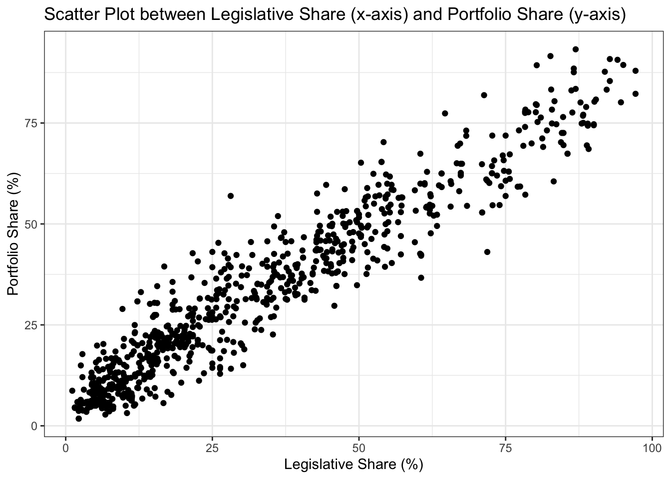
Looking at the scatter plot, we observe a positive association between the two variables. Higher values of legislative_share tend to be associated with higher values of portfolio_share. In addition, we notice that the relationship between the two variables appears to be strongly linear. In the previous chapter, we investigated the direction and strength of the linear association computing the correlation coefficient. Now, we want to fit a linear model to summarize their relationship.
Based on our sample data, this fitted line can be represented by its estimated systematic component \(\widehat{Y}_i\) and its estimated stochastic or random component \(\widehat\epsilon_i\):
Estimated systematic component: \[ \widehat{p}_{i} = \widehat{\alpha} + \widehat{\beta} s_{i} \]
Estimated stochastic component: \[ \widehat{\epsilon}_{i} = p_{i} - \widehat{p}_{i} \]
To calculate the coefficients of the linear model using the least squares method in R, we employ the lm() function, which stands for ‘linear model.’ This function requires specifying a formula of the form Y ~ X, where Y represents the dependent variable, and X represents the independent variable.To fit a line summarizing the linear relationship between legislative_share and portfolio_share, we execute the following code (notice that we are also storing it as an object called coalitions_model):
# Fit and store a linear model between legislative_share and portfolio_share
coalitions_model <- lm(portfolio_share ~ legislative_share, data = coalitions)
coalitions_model
##
## Call:
## lm(formula = portfolio_share ~ legislative_share, data = coalitions)
##
## Coefficients:
##       (Intercept)  legislative_share
##            5.1998             0.8434
In the output from the lm() function above, you can observe that the estimated intercept \(\widehat\alpha\) is 5.20, while the estimated slope \(\widehat\beta\) is 0.84.
8.3 Interpreting the Results of a Regression Model
How should we interpret \(\widehat\alpha = 5.20\) from our linear model? \(\widehat\alpha\) represents the predicted value of \(p\), denoted as \(\hat{p}\), when \(s\) is zero. In the context of our variables, portfolio_share and legislative_share (both measured in percentages), this estimated intercept suggests that when legislative_share is zero, we predict, on average, a portfolio_share of 5.20. It’s important to note that the interpretation of the intercept may not always hold practical significance, particularly when the range of observed values of the predictor doesn’t include zero. In our example, a party with zero legislative seats wouldn’t typically be part of a coalition government because the primary incentive for coalition formation is gaining legislative support in exchange for portfolios from parties with representation in the legislature. In fact, there is no coalition party in our data set with a legislative_share of zero; the lowest observed value is 1.78, roughly equivalent to a coalition party contributing 2% of the legislative seats controlled by the coalition in the legislature. Remember: It’s essential to thoroughly explore your data before running regression analysis to understand your variables and their practical implications.
How should we interpret \(\widehat\beta = 0.84\)? The value of \(\widehat\beta\) represents the change in \(\widehat{Y}\) associated with a one-unit increase in \(X\), denoted as \(\Delta\widehat{Y}\) associated with \(\Delta\hat{X} = 1\). In our example, where \(Y\) is portfolio_share and \(X\) is legislative_share (both measured in percentages), we interpret the estimated slope coefficient as indicating that a one-percentage-point increase in legislative_share is associated with a predicted increase in portfolio_share of 0.84 percentage points, on average.
As we discussed in Week 8, we can easily add the fitted line to the previously produced scatter plot using the geom_smooth() function in ggplot2 with the parameter method = "lm" (lm stands for linear model).
# Fitting the predicted line to the scatter plot
ggplot(coalitions, aes(x = legislative_share, y = portfolio_share)) +
geom_point() +
geom_smooth(method = "lm", se = FALSE) + # se = FALSE for no confidence interval around the line
labs(y = "Portfolio Share (%)",
x = "Legislative Share (%)",
title = "Scatter Plot with Fitted Line Representing the Linear Association Between Legislative Share and Portfolio Share") +
theme_few()
## `geom_smooth()` using formula = 'y ~ x'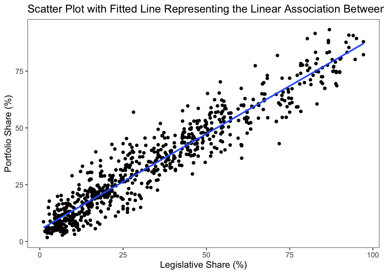
In the resulting figure, we can observe that the data points are closely clustered around the fitted line. This reinforces the strong linear association we previously identified through both our correlation analysis (see Section 6.4 in the last chapter) and the estimated \(\beta\) from our linear regression model. The slight deviation of data points from the line aligns with the value of \(\widehat\beta\) we found, which is smaller than 1 (\(\widehat\beta = 0.84\)). In essence, while there is a strong positive linear association between legislative_share and portfolio_share, suggesting that the more legislative seats the coalition parties contribute to the coalition government, the more portfolios they receive on a proportional basis, this relationship is not perfect.
Generally speaking, there are usually two types of predictions we are interested in making.
First, we may want to predict the average value of the outcome variable given a value of the predictor—i.e., computing \(\widehat{Y}\) based on X. When this is the case, we plug the value of X into the predicted linear model and calculate \(\widehat{Y}\):
\[ \widehat{Y} = \widehat{\alpha} + \widehat{\beta} X \]
For instance, let’s say we want to predict the value of portfolio_share (our dependent variable p) when legislative_share (our independent variable s) is at its minimum value. As outlined above, this minimum value is 1.78. Given this, what would be our best estimate for portfolio_share when legislative_share is 1.78? To answer this, we look to the relationship we previously estimated between these variables. By plugging 1.78 into the value of s in our predicted linear model, we can predict the corresponding portfolio_share:
\[ \begin{aligned} \widehat{p} &= 5.20 + 0.84 \, s \\ &= 5.20 + 0.84 \times 1.78 \\ &= 6.6952 \end{aligned} \] We are now ready to conduct statistical inference (i.e., make predictions about a population based on a sample of data from that population): We predict that, on average, a coalition party contributing 1.78% of the legislative seats in a coalition controls approximately 6.7% of the available portfolios in the government. In a perfectly proportional distribution scenario, we would expect this coalition party to control close to 2% of the available portfolios. The discrepancy we observed indicates a disproportionate allocation of portfolios, favoring coalition parties that contribute a smaller proportion of legislative seats. There may be underlying factors not captured in our current model that contribute to this observation. For instance, a party might possess a higher bargaining power during the coalition government formation process, or it might hold a strategically important position that grants it more influence in portfolio allocation, even if it doesn’t bring in a substantial number of legislative seats. We will explore these complexities in greater detail in the next chapter, using multivariate regression analysis.
Second, we may want to predict the average change in the outcome variable associated with a change in the value of the predictor. When this is the case, we use the formula that computes the change in the predicted outcome (denoted as \(\Delta\widehat{Y}\) ) associated with a one unit increase in X (denoted as \(\Delta X = 1\) ), given by:
\[ \Delta\widehat{Y} = \widehat{\beta} \Delta X \]
For example, suppose we aim to predict the change in portfolio_share resulting from a 10 percentage point increase in legislative_share. This involves estimating \(\Delta\hat{p}\) when legislative_share increases by 10% (\(\Delta s = 10\)). Since both our dependent and independent variables are in percentage terms, their metric interpretation remains consistent. To compute the change, we use the formula for the predicted change in portfolio_share and plug in the value of change in legislative_share:
\[ \begin{aligned} \Delta\widehat{p} &= 0.84 \Delta s \\ &= 0.84 \times 10 \\ &= 8.4 \end{aligned} \] From our fitted linear model, we infer that, on average, a 10% increase in legislative_share is associated with an approximate 8% increase in portfolio_share.
To further assess the substantive implications of our results, we should first evaluate the statistical significance of our estimated coefficients, which we will cover in the next section.
8.4 Statistical vs. Substantive Significance
The lm() function is a very easy way to conduct a linear regression model in R. It’s output, on the other hand is very limited, restricted to the presentation of the coefficients. Neverthless, once you’ve fitted a linear model using lm(), there are several functions and commands you can use to extract and examine important information about your model. Below I present a non-exhaustive list of commonly used functions and what they provide.
The coef() function retrieves the estimated coefficients of the model, \(\widehat\alpha\) and \(\widehat\beta\):
coef(coalitions_model) # retrieves the coefficients
##       (Intercept) legislative_share
##         5.1997595         0.8434252
The fitted() function retrieves the fitted values (i.e., predicted values) of the dependent variable \(\widehat{Y}_i\) for the data used in the model. For each observation in the dataset, there’s a corresponding predicted value based on the model’s coefficients and the values of the predictor variable \(X_i\). As a consequence, the number of fitted values is equal to the number of observations in the data set. Given the extensive list of values that would be displayed in the R console, we are omitting the output in this instance. However, you can execute the code on your local machine to view the results.
The residuals() function retrieves the differences between the observed and predicted values for the dependent variable (i.e., \(\widehat\epsilon_{i}\) ). Since there’s a predicted (fitted) value (\(\widehat{Y}_i\) ) and an actual (original) value (\(Y_i\) ) for each observation in our dependent variable, there will be a residual for each observation as well. In other words, because we calculate a residual for each observed value in the data set, the number of residuals is equal to the number of observations. Given the extensive list of values that would be displayed, we are also omitting the output in this instance.
The confint() function computes confidence intervals for one or more model parameters. This gives a range within which the true parameter value is expected to fall with a certain level of confidence.
confint(coalitions_model, level = 0.95) # retrieves the confidence intervals of the coefficients at 95% level of confidence
##                       2.5 %    97.5 %
## (Intercept)       4.4481761 5.9513428
## legislative_share 0.8252206 0.8616297
Among the functions in R for summarizing linear model results, summary() stands out as the most commonly employed. It provides a structured and interpretable overview of the model’s results. Users benefit from its comprehensive output, without needing to extract individual metrics or resort to multiple functions.
summary(coalitions_model) # summary statistics from the linear model
##
## Call:
## lm(formula = portfolio_share ~ legislative_share, data = coalitions)
##
## Residuals:
##      Min       1Q   Median       3Q      Max
## -22.7612  -3.9262  -0.4303   3.7316  28.0192
##
## Coefficients:
##                   Estimate Std. Error t value Pr(>|t|)
## (Intercept)       5.199759   0.382891   13.58   <2e-16 ***
## legislative_share 0.843425   0.009274   90.94   <2e-16 ***
## ---
## Signif. codes:  0 '***' 0.001 '**' 0.01 '*' 0.05 '.' 0.1 ' ' 1
##
## Residual standard error: 6.462 on 805 degrees of freedom
## Multiple R-squared:  0.9113, Adjusted R-squared:  0.9112
## F-statistic:  8271 on 1 and 805 DF,  p-value: < 2.2e-16
Although the summary() function retrieves several important pieces of information (discussed later in the course), below we will focus on a few specific ones that are essential for the interpretation of the main results of our model and are also commonly featured in academic papers. Specifically, we will focus on the residuals, the estimated coefficients and their statistical significance, and the model’s goodness-of-fit measure \((R^{2})\).
- Residuals: Focusing on the residuals, which represent the differences between the observed values of the dependent variable (portfolio_share) and the predictions made by our linear model, we scrutinize the residuals’ size and distribution, as they can highlight potential areas where the model might not adequately capture the underlying dynamics of the relationship of interest.
- The minimum residual value is \(-22.7612\), indicating that the model overpredicted the portfolio_share by approximately 22.76 units for at least one observation.
- On the other end, the maximum residual value is \(28.0192\), indicating that the model underpredicted the portfolio_share by around 28.02 units for at least one observation.
- The median residual is \(-0.4303\), which is close to zero. This indicates that the central tendency of the model’s prediction errors is small, suggesting that the model’s predictions align closely with the observed values for many data points.
- The interquartile range, which spans from the 1st quartile to the 3rd quartile residuals, is roughly \(7.7\) (i.e., \(3.7316 - (-3.9262)\)). This metric provides a sense of the spread of the middle 50% of residuals, illuminating the variability in the model’s fit across different observations. Hence, 50% of the model’s residuals are between -3.9262 and 3.7316 units. In simpler terms, for half of our data points, the model’s predictions for the dependent variable deviate from the actual observations by an amount that can vary up to roughly 7.7 units. Given that our unit of measurement is percentage points, the model’s predictions of portfolio_share based on legislative_share for half of the coalition parties could be off by up to 7.7%, either as an overestimate or an underestimate.
- The minimum residual value is \(-22.7612\), indicating that the model overpredicted the portfolio_share by approximately 22.76 units for at least one observation.
The “Coefficients” section is a critical component of the summary() output for a linear regression model in R, providing information about:
- Estimated Coefficients: The first column (“Estimate”) of the “Coefficients:” section retrieves the estimated parameters \(\widehat\alpha\) (referred to as the Intercept) and \(\widehat\beta\) for each predictor, with our two-variable regression analysis focusing solely on legislative_share. These estimated values should be the same as those displayed in the
lm()function’s output.
- Intercept = 5.199759: The intercept represents the estimated percentage of portfolios controlled by coalition parties when the percentage of legislative seats the coalition party contributes to the coalition government is zero. In this context, it suggests that when a coalition party contributes no legislative seats, they are estimated to control approximately 5.20% of portfolios. However, as above discussed, this value should be interpreted cautiously as it might not have a practical meaning in some contexts.
- Legislative_Share = 0.843425: The coefficient for legislative_share represents the estimated change in the percentage of portfolios controlled by a coalition party for every one-unit increase in their contribution to legislative seats in the coalition government. In this case, it indicates that, on average, for each additional percentage point of legislative seats contributed, the party is estimated to control approximately 0.84% more portfolios. (For a detailed discussion of the estimates, please see the previous section.)
- Intercept = 5.199759: The intercept represents the estimated percentage of portfolios controlled by coalition parties when the percentage of legislative seats the coalition party contributes to the coalition government is zero. In this context, it suggests that when a coalition party contributes no legislative seats, they are estimated to control approximately 5.20% of portfolios. However, as above discussed, this value should be interpreted cautiously as it might not have a practical meaning in some contexts.
- Statistical Significance: To evaluate the statistical significance of our estimates, we rely on the remaining information presented in the “Coefficients:” section: Std. Error, t value, and Pr(>|t|). Remember that, when evaluating the statistical significance of an estimated parameter, we often employ q hypothesis testing. Hypothesis testing helps us make informed inferences about the relationships and effects we observe in our data. This usually involves comparing our estimated coefficient for a predictor variable against a null hypothesis. In the case of a linear regression model, the null hypothesis, typically tested at a chosen level of confidence (often 95% in most academic journals), posits that the coefficient (parameter) associated with a predictor variable is equal to zero. In other words, this means that the predictor variable does not seem to be associated with the dependent variable and that the value we obtained for the estimated coefficient is likely a result of random chance rather than an association between the variables in the broader population.
Conversely, when we find support for the alternative hypothesis, it indicates that the coefficient associated with the predictor variable is different from zero. When conducting our hypothesis test usingsummary(), then, we’re essentially considering two potential scenarios: either the parameter is not significantly different from zero, or it’s significantly different from zero. This practice, commonly employed in regression analysis, is referred to as a two-tailed hypothesis test. This approach enables us to evaluate the statistical significance of the relationship in both directions without assuming a specific direction of effect. In simpler terms, it allows us to determine whether a predictor variable seems unrelated to the dependent variable (a coefficient close to zero) or whether it indeed influences the dependent variable (different from zero), without assuming a specific positive or negative direction of effect. We will explore this concept in greater detail in the upcoming chapter.
- Standard Error: The “Std. Error” column provides the standard error associated with each coefficient estimate. This value quantifies the degree of uncertainty or imprecision in the estimate. Smaller standard errors indicate more precise and reliable coefficient estimates, while larger ones imply greater uncertainty. For detailed guidance on calculating the standard error, please refer to section 6.3: Exploring Data and One Variable At a Time in this book and the Week 6 slides.
- t value: The “t value” column displays the t-statistic for each coefficient. This statistic is calculated by dividing the estimated coefficient by its standard error, and it measures how many standard errors the estimated coefficient is away from zero. Larger absolute t-values indicate that the coefficient is further from zero, which, when compared to the critical t-value associated with a specific level of confidence (often obtained from a t-distribution table), provides evidence against the null hypothesis.
- Pr(>|t|): The “Pr(>|t|)” column shows the p-value associated with each coefficient. The p-value assesses the likelihood of observing a t-statistic as extreme as the one calculated, assuming that the true coefficient in the population is zero (i.e., no effect). In most cases, these are the informed conclusions we can draw when evaluating the p-value:
- Small p-values (usually below 0.05): Small p-values provide evidence against the null hypothesis and lend support to the alternative hypothesis. In other words, it means that the observed result is unlikely to occur by random chance if the null hypothesis were true. Consequently, you can conclude that the relationship you observed between the variables or the effect of the independent variable on the dependent variable you found is statistically significant. As a quick visual indicator of statistical significance, the
summary()output relies on stars (or more precisely, asterisks) placed beside coefficients. For example, “*” represents statistical significance at the conventional 95% confidence level, while “***” represents statistical significance at the higher 99% level, encompassing the conventional threshold. The ‘Signif. codes’ column assigns the following symbols for different confidence levels: “***” for \(p < 0.001\), “**” for \(p < 0.01\), “*” for \(p < 0.05\), and “.” for \(p < 0.1\).
- Large p-values (usually above 0.05): Conversely, when the p-value is large, it suggests that the observed result is quite likely to occur even if the null hypothesis is true. In other words, there isn’t enough evidence to conclude that the effect or relationship is statistically significant. Instead, it is possible that the observed result could be due to randomness. Being honest and transparent about the results of hypothesis tests, even when they reveal a non-significant relationship between variables, is of paramount importance in scientific research. This practice upholds scientific integrity by presenting findings as they are, without manipulation. Furthermore, it contributes to the collective body of knowledge, as non-significant results can offer valuable insights and guide future research.
- Small p-values (usually below 0.05): Small p-values provide evidence against the null hypothesis and lend support to the alternative hypothesis. In other words, it means that the observed result is unlikely to occur by random chance if the null hypothesis were true. Consequently, you can conclude that the relationship you observed between the variables or the effect of the independent variable on the dependent variable you found is statistically significant. As a quick visual indicator of statistical significance, the
- \(R^2\) Diagnostic Metric (Multiple R-squared):
- The \(R^2\) statistic, also known as the multiple R-squared, is a statistical measure that represents the proportion of the variance in the dependent variable (in our example, percentage of portfolios controlled by coalition parties) that is explained by the independent variables (percentage of legislative seats contributed to the coalition government). In simple terms, this metric indicates how well the model fits the data (also referred to as the goodness-of-fit measure of the model). The basic idea of the \(R^2\)statistic is shown in Figure 7.1 below, which is a Venn diagram depiction of variation in \(X\) and \(Y\) as well as covariation between \(X\) and \(Y\).
The idea behind the diagram is to represent the variation in each variable using circles. The size of each circle corresponds to the magnitude of variation in the respective variable. In the figure above, the variation in \(Y\) is divided into two areas, \(a\) and \(b\), while the variation in \(X\) is divided into areas \(b\) and \(c\). Specifically, area \(a\) represents the variation in \(Y\) that is not related to variation in \(X\), while area \(b\), the intersection between areas \(a\) and \(c\), represents covariation between \(X\) and \(Y\). In a two-variable regression model, area \(a\) is the residual or stochastic variation in \(Y\). The \(R^2\) statistic is determined by dividing area \(b\) by the sum of areas \(a\) and \(b\)—this sum represents the total variation in \(Y\). Therefore, when area \(a\) becomes smaller and area \(b\) becomes larger, the \(R^2\) value becomes larger.
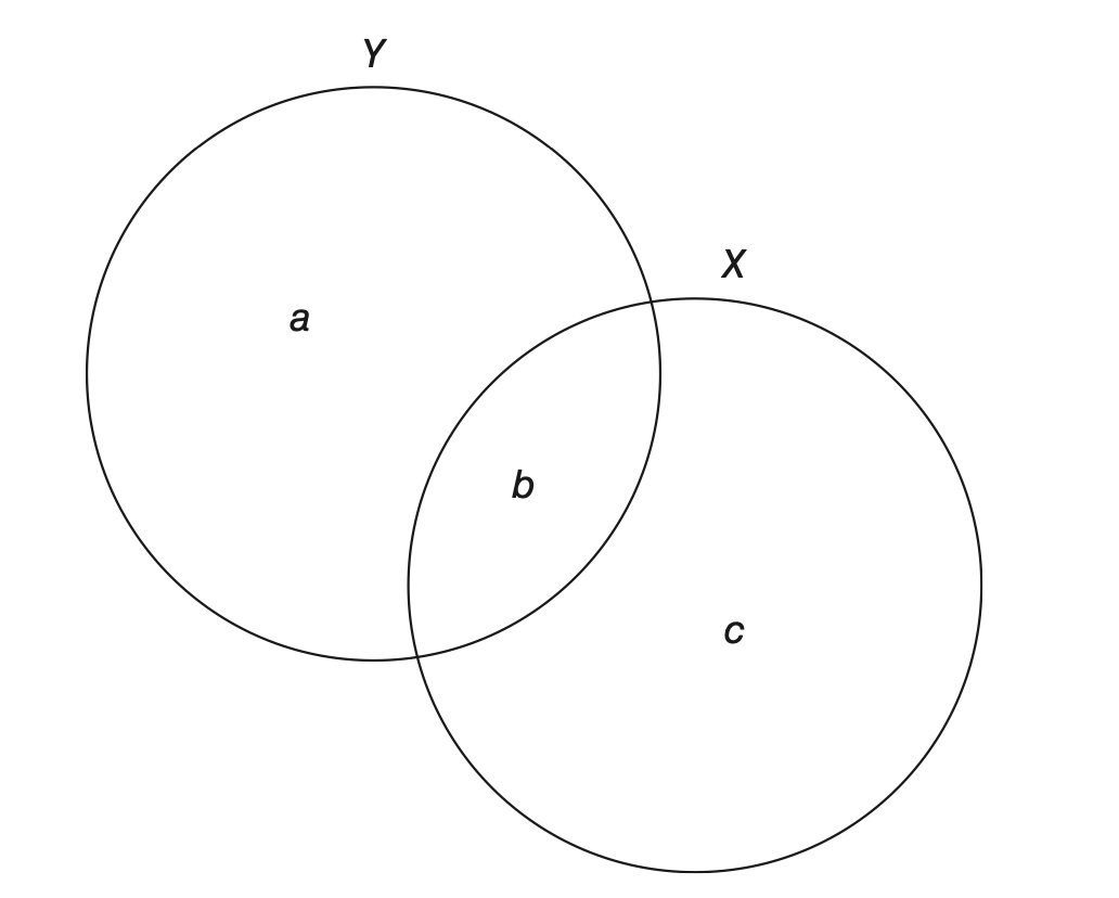
Figure 8.1: Venn Diagram of Variance and Covariance for X and Y
\(R^2\) values range from 0 to 1, where: An \(R^2\) of 0 means that the model explains none of the variance in the dependent variable, indicating a poor fit, and an \(R^2\) of 1 means that the model explains all of the variance in the dependent variable, indicating a perfect fit. In the model we conducted, the \(R^2\) value is approximately 0.91, which means that approximately 91% of the variation in portfolio control can be explained by the percentage of legislative seats contributed by coalition parties. This is a high value and suggests that our model is a good fit for the data. In other words, it suggests that the single predictor included in our model explains a large proportion of the variability in the dependent variable—i.e, the variation in portfolio_share can be largely attributed to changes in legislative_share.
- The \(R^2\) statistic, also known as the multiple R-squared, is a statistical measure that represents the proportion of the variance in the dependent variable (in our example, percentage of portfolios controlled by coalition parties) that is explained by the independent variables (percentage of legislative seats contributed to the coalition government). In simple terms, this metric indicates how well the model fits the data (also referred to as the goodness-of-fit measure of the model). The basic idea of the \(R^2\)statistic is shown in Figure 7.1 below, which is a Venn diagram depiction of variation in \(X\) and \(Y\) as well as covariation between \(X\) and \(Y\).
Now, that we are more confident about the statistical significance of our results, we can provide some substantive significance for them. Substantive significance, in contrast to statistical significance, refers to the practical or real-world importance or meaningfulness of a finding or result. While statistical significance focuses on whether an observed effect is likely to be the result of a true relationship or if it could have occurred by random chance, substantive significance provides the actual impact or relevance of that effect in a broader context. When considering the real-world implications and consequences of an observed effect, we usually have in mind questions such as: Does the observed change or relationship we found have practical importance? How does it change the field of study? How does it change the way we see the world?
For instance, knowing how portfolios are allocated in the coalition government formation process bears major implications for the distribution of power among political elites (i.e., who gets to govern), how governments formulate and enact public policies, the duration of governments, and the electoral fate of political parties.
With the results of the linear regression analysis we just conducted at hand, we can infer from the statistically significant relationship between the share of portfolios controlled by coalition parties and the share of legislative seats they contribute within coalition governments that as coalition parties gain more influence in terms of legislative seats, they also gain a larger share of portfolios within the government’s executive power. In our study, we also found support for Gamson’s law. Although not perfect, the distribution of portfolios among coalition parties seems to be very proportional to their contribution in legislative seats. As a result, on average, and with parliamentary democracies in mind, the balance of power in executive coalition cabinets appears to reflect the balance of power in the legislature. A prolific body of literature has been produced with this evidence in mind. Gamson’s law has been tested in different countries, over different time periods, and under different forms of government.
If you are interested to read more about this topic, you can check out my new article which addresses the research question: When and why should we expect similarities and differences in the dynamics of coalition formation between presidential and parliamentary democracies, and in particular within presidential systems?
8.5 Interactive R Learning: Lab 7
By now, swirl should be installed on your machine (refer to Section 1.6 if you’re unsure).
There’s no need to reinstall the qss-swirl lessons. Simply commence a qss-swirl lesson after loading the swirl package.
In Lab 7, we’ll work on “Lesson 8: PREDICTION2,” which serves as a companion to “Chapter 4: Prediction” from our required book, QSS.